Dijkstra 最短路径算法

https://labuladong.github.io/algo/2/19/41/

其实，很多算法的底层原理异常简单，无非就是一步一步延伸，变得看起来好像特别复杂，特别牛逼。

但如果你看过历史文章，应该可以对算法形成自己的理解，就会发现很多算法都是换汤不换药，毫无新意，非常枯燥。

比如，我们说二叉树非常重要，你把这个结构掌握了，就会发现 动态规划， 分治算法， 回溯（DFS）算法， BFS 算法框架， Union-Find 并查集算法， 二叉堆实现优先级队列 就是把二叉树翻来覆去的运用。

那么本文又要告诉你，Dijkstra 算法（一般音译成迪杰斯特拉算法）无非就是一个 BFS 算法的加强版，它们都是从二叉树的层序遍历衍生出来的。

这也是为什么我在 学习数据结构和算法的框架思维 中这么强调二叉树的原因。

下面我们由浅入深，从二叉树的层序遍历聊到 Dijkstra 算法，给出 Dijkstra 算法的代码框架，顺手秒杀几道运用 Dijkstra 算法的题目。

图的抽象

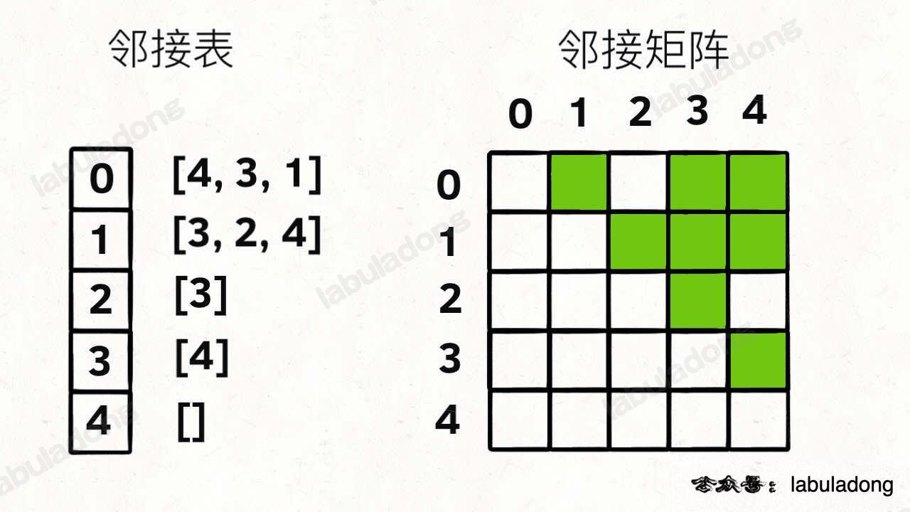
前文 图论第一期：遍历基础 说过「图」这种数据结构的基本实现，图中的节点一般就抽象成一个数字（索引），图的具体实现一般是「邻接矩阵」或者「邻接表」。

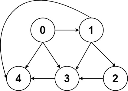
比如上图这幅图用邻接表和邻接矩阵的存储方式如下：

前文 图论第二期：拓扑排序 告诉你，我们用邻接表的场景更多，结合上图，一幅图可以用如下 Java 代码表示：

// graph[s] 存储节点 s 指向的节点（出度）
List<Integer>[] graph;

如果你想把一个问题抽象成「图」的问题，那么首先要实现一个 API adj：

// 输入节点 s 返回 s 的相邻节点
List<Integer> adj(int s);

类似多叉树节点中的 children 字段记录当前节点的所有子节点，adj(s) 就是计算一个节点 s 的相邻节点。

比如上面说的用邻接表表示「图」的方式，adj 函数就可以这样表示：

List<Integer>[] graph;

// 输入节点 s，返回 s 的相邻节点
List<Integer> adj(int s) {
    return graph[s];
}

当然，对于「加权图」，我们需要知道两个节点之间的边权重是多少，所以还可以抽象出一个 weight 方法：

// 返回节点 from 到节点 to 之间的边的权重
int weight(int from, int to);

这个 weight 方法可以根据实际情况而定，因为不同的算法题，题目给的「权重」含义可能不一样，我们存储权重的方式也不一样。

有了上述基础知识，就可以搞定 Dijkstra 算法了，下面我给你从二叉树的层序遍历开始推演出 Dijkstra 算法的实现。

二叉树层级遍历和 BFS 算法

我们之前说过二叉树的层级遍历框架：

// 输入一棵二叉树的根节点，层序遍历这棵二叉树
void levelTraverse(TreeNode root) {
    if (root == null) return 0;
    Queue<TreeNode> q = new LinkedList<>();
    q.offer(root);

    int depth = 1;
    // 从上到下遍历二叉树的每一层
    while (!q.isEmpty()) {
        int sz = q.size();
        // 从左到右遍历每一层的每个节点
        for (int i = 0; i < sz; i++) {
            TreeNode cur = q.poll();
            printf("节点 %s 在第 %s 层", cur, depth);

            // 将下一层节点放入队列
            if (cur.left != null) {
                q.offer(cur.left);
            }
            if (cur.right != null) {
                q.offer(cur.right);
            }
        }
        depth++;
    }
}

我们先来思考一个问题，注意二叉树的层级遍历 while 循环里面还套了个 for 循环，为什么要这样？

while 循环和 for 循环的配合正是这个遍历框架设计的巧妙之处：

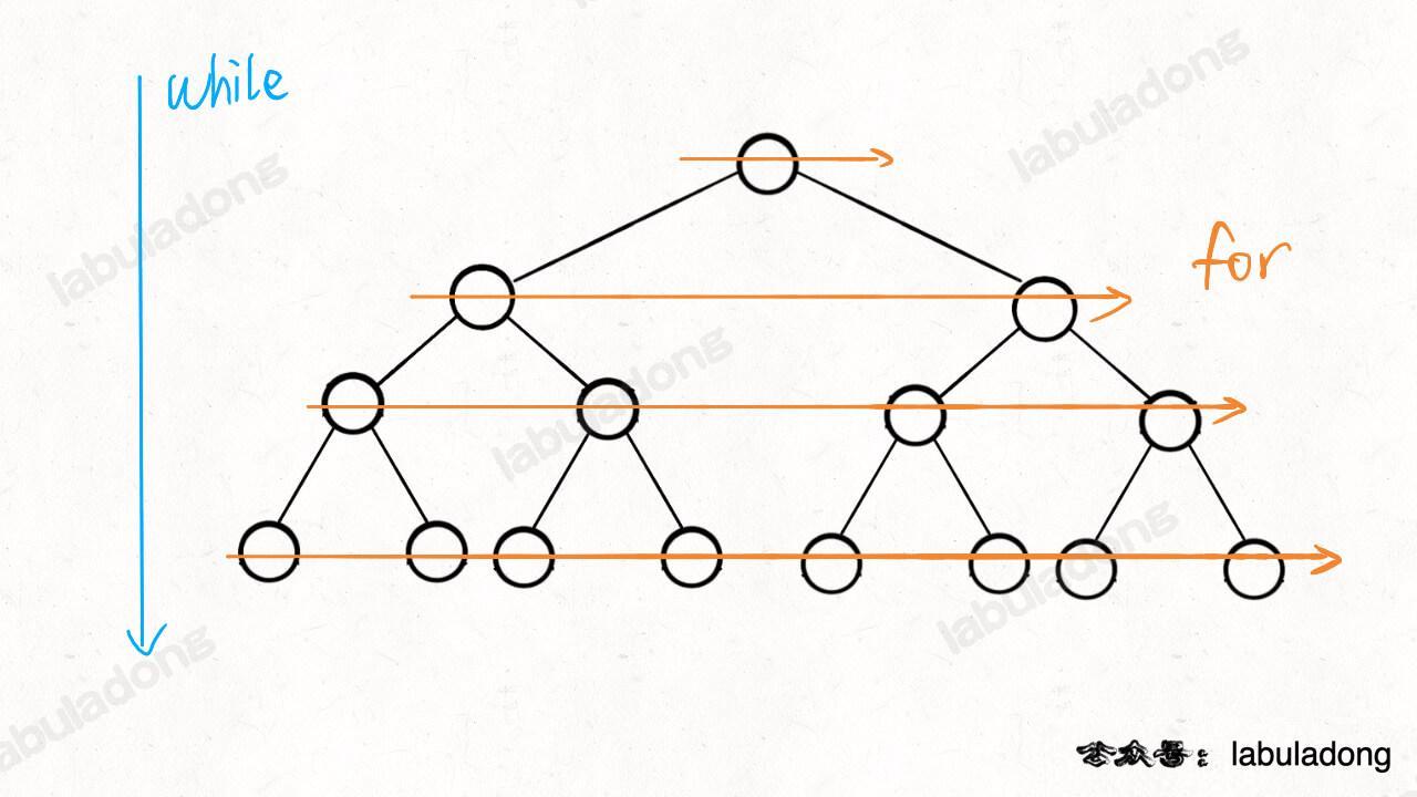
while 循环控制一层一层往下走，for 循环利用 sz 变量控制从左到右遍历每一层二叉树节点。

注意我们代码框架中的 depth 变量，其实就记录了当前遍历到的层数。换句话说，每当我们遍历到一个节点 cur，都知道这个节点属于第几层。

算法题经常会问二叉树的最大深度呀，最小深度呀，层序遍历结果呀，等等问题，所以记录下来这个深度 depth 是有必要的。

基于二叉树的遍历框架，我们又可以扩展出多叉树的层序遍历框架：

// 输入一棵多叉树的根节点，层序遍历这棵多叉树
void levelTraverse(TreeNode root) {
    if (root == null) return;
    Queue<TreeNode> q = new LinkedList<>();
    q.offer(root);

    int depth = 1;
    // 从上到下遍历多叉树的每一层
    while (!q.isEmpty()) {
        int sz = q.size();
        // 从左到右遍历每一层的每个节点
        for (int i = 0; i < sz; i++) {
            TreeNode cur = q.poll();
            printf("节点 %s 在第 %s 层", cur, depth);

            // 将下一层节点放入队列
            for (TreeNode child : cur.children) {
                q.offer(child);
            }
        }
        depth++;
    }
}

基于多叉树的遍历框架，我们又可以扩展出 BFS（广度优先搜索）的算法框架：

// 输入起点，进行 BFS 搜索
int BFS(Node start) {
    Queue<Node> q; // 核心数据结构
    Set<Node> visited; // 避免走回头路
    
    q.offer(start); // 将起点加入队列
    visited.add(start);

    int step = 0; // 记录搜索的步数
    while (q not empty) {
        int sz = q.size();
        /* 将当前队列中的所有节点向四周扩散一步 */
        for (int i = 0; i < sz; i++) {
            Node cur = q.poll();
            printf("从 %s 到 %s 的最短距离是 %s", start, cur, step);

            /* 将 cur 的相邻节点加入队列 */
            for (Node x : cur.adj()) {
                if (x not in visited) {
                    q.offer(x);
                    visited.add(x);
                }
            }
        }
        step++;
    }
}

如果对 BFS 算法不熟悉，可以看前文 BFS 算法框架，这里只是为了让你做个对比，所谓 BFS 算法，就是把算法问题抽象成一幅「无权图」，然后继续玩二叉树层级遍历那一套罢了。

注意，我们的 BFS 算法框架也是 while 循环嵌套 for 循环的形式，也用了一个 step 变量记录 for 循环执行的次数，无非就是多用了一个 visited 集合记录走过的节点，防止走回头路罢了。

为什么这样呢？

所谓「无权图」，与其说每条「边」没有权重，不如说每条「边」的权重都是 1，从起点 start 到任意一个节点之间的路径权重就是它们之间「边」的条数，那可不就是 step 变量记录的值么？

再加上 BFS 算法利用 for 循环一层一层向外扩散的逻辑和 visited 集合防止走回头路的逻辑，当你每次从队列中拿出节点 cur 的时候，从 start 到 cur 的最短权重就是 step 记录的步数。

但是，到了「加权图」的场景，事情就没有这么简单了，因为你不能默认每条边的「权重」都是 1 了，这个权重可以是任意正数（Dijkstra 算法要求不能存在负权重边），比如下图的例子：

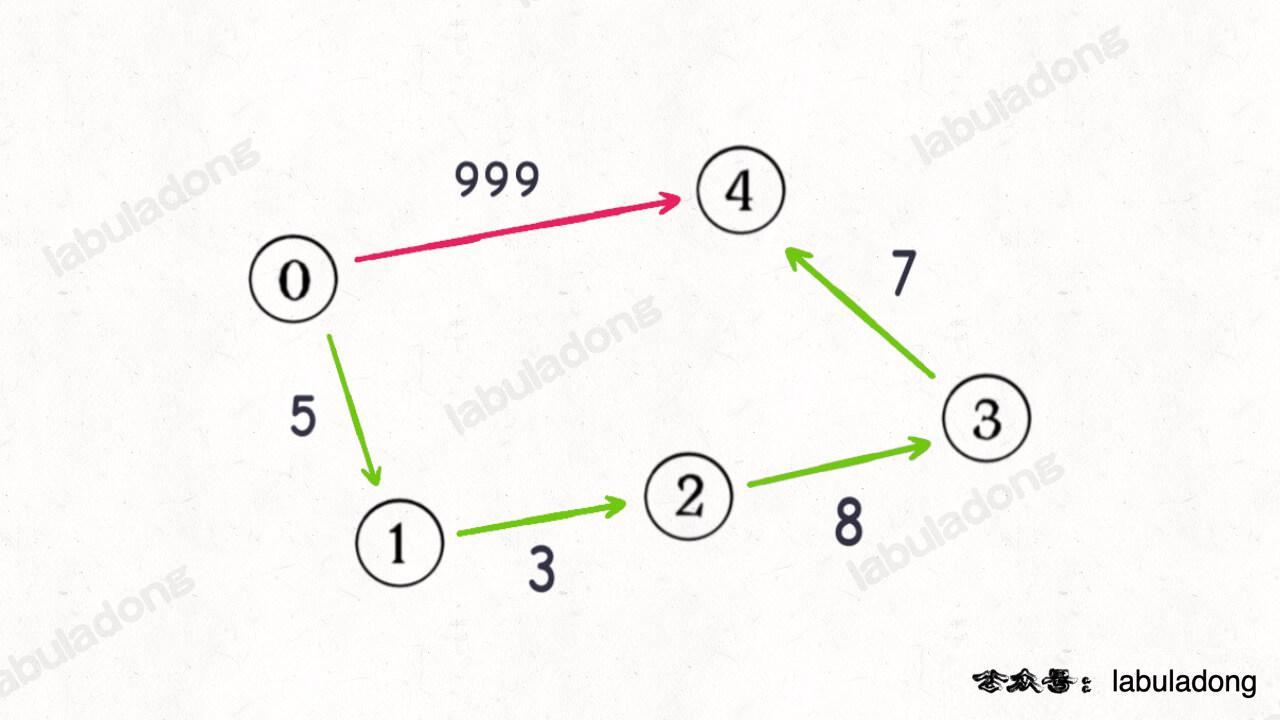
如果沿用 BFS 算法中的 step 变量记录「步数」，显然红色路径一步就可以走到终点，但是这一步的权重很大；正确的最小权重路径应该是绿色的路径，虽然需要走很多步，但是路径权重依然很小。

其实 Dijkstra 和 BFS 算法差不多，不过在讲解 Dijkstra 算法框架之前，我们首先需要对之前的框架进行如下改造：

想办法去掉 while 循环里面的 for 循环。

为什么？有了刚才的铺垫，这个不难理解，刚才说 for 循环是干什么用的来着？

是为了让二叉树一层一层往下遍历，让 BFS 算法一步一步向外扩散，因为这个层数 depth，或者这个步数 step，在之前的场景中有用。

但现在我们想解决「加权图」中的最短路径问题，「步数」已经没有参考意义了，「路径的权重之和」才有意义，所以这个 for 循环可以被去掉。

怎么去掉？就拿二叉树的层级遍历来说，其实你可以直接去掉 for 循环相关的代码：

// 输入一棵二叉树的根节点，遍历这棵二叉树所有节点
void levelTraverse(TreeNode root) {
    if (root == null) return 0;
    Queue<TreeNode> q = new LinkedList<>();
    q.offer(root);

    // 遍历二叉树的每一个节点
    while (!q.isEmpty()) {
        TreeNode cur = q.poll();
        printf("我不知道节点 %s 在第几层", cur);

        // 将子节点放入队列
        if (cur.left != null) {
            q.offer(cur.left);
        }
        if (cur.right != null) {
            q.offer(cur.right);
        }
    }
}

但问题是，没有 for 循环，你也没办法维护 depth 变量了。

如果你想同时维护 depth 变量，让每个节点 cur 知道自己在第几层，可以想其他办法，比如新建一个 State 类，记录每个节点所在的层数：

class State {
    // 记录 node 节点的深度
    int depth;
    TreeNode node;

    State(TreeNode node, int depth) {
        this.depth = depth;
        this.node = node;
    }
}

// 输入一棵二叉树的根节点，遍历这棵二叉树所有节点
void levelTraverse(TreeNode root) {
    if (root == null) return 0;
    Queue<State> q = new LinkedList<>();
    q.offer(new State(root, 1));

    // 遍历二叉树的每一个节点
    while (!q.isEmpty()) {
        State cur = q.poll();
        TreeNode cur_node = cur.node;
        int cur_depth = cur.depth;
        printf("节点 %s 在第 %s 层", cur_node, cur_depth);

        // 将子节点放入队列
        if (cur_node.left != null) {
            q.offer(new State(cur_node.left, cur_depth + 1));
        }
        if (cur_node.right != null) {
            q.offer(new State(cur_node.right, cur_depth + 1));
        }
    }
}

这样，我们就可以不使用 for 循环也确切地知道每个二叉树节点的深度了。

如果你能够理解上面这段代码，我们就可以来看 Dijkstra 算法的代码框架了。

Dijkstra 算法框架

首先，我们先看一下 Dijkstra 算法的签名：

// 输入一幅图和一个起点 start，计算 start 到其他节点的最短距离
int[] dijkstra(int start, List<Integer>[] graph);

输入是一幅图 graph 和一个起点 start，返回是一个记录最短路径权重的数组。

比方说，输入起点 start = 3，函数返回一个 int[] 数组，假设赋值给 distTo 变量，那么从起点 3 到节点 6 的最短路径权重的值就是 distTo[6]。

是的，标准的 Dijkstra 算法会把从起点 start 到所有其他节点的最短路径都算出来。

当然，如果你的需求只是计算从起点 start 到某一个终点 end 的最短路径，那么在标准 Dijkstra 算法上稍作修改就可以更高效地完成这个需求，这个我们后面再说。

其次，我们也需要一个 State 类来辅助算法的运行：

class State {
    // 图节点的 id
    int id;
    // 从 start 节点到当前节点的距离
    int distFromStart;

    State(int id, int distFromStart) {
        this.id = id;
        this.distFromStart = distFromStart;
    }
}

类似刚才二叉树的层序遍历，我们也需要用 State 类记录一些额外信息，也就是使用 distFromStart 变量记录从起点 start 到当前这个节点的距离。

刚才说普通 BFS 算法中，根据 BFS 的逻辑和无权图的特点，第一次遇到某个节点所走的步数就是最短距离，所以用一个 visited 数组防止走回头路，每个节点只会经过一次。

加权图中的 Dijkstra 算法和无权图中的普通 BFS 算法不同，在 Dijkstra 算法中，你第一次经过某个节点时的路径权重，不见得就是最小的，所以对于同一个节点，我们可能会经过多次，而且每次的 distFromStart 可能都不一样，比如下图：

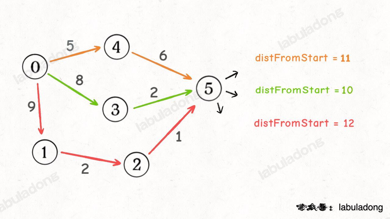
我会经过节点 5 三次，每次的 distFromStart 值都不一样，那我取 distFromStart 最小的那次，不就是从起点 start 到节点 5 的最短路径权重了么？

好了，明白上面的几点，我们可以来看看 Dijkstra 算法的代码模板。

其实，Dijkstra 可以理解成一个带 dp table（或者说备忘录）的 BFS 算法，伪码如下：

// 返回节点 from 到节点 to 之间的边的权重
int weight(int from, int to);

// 输入节点 s 返回 s 的相邻节点
List<Integer> adj(int s);

// 输入一幅图和一个起点 start，计算 start 到其他节点的最短距离
int[] dijkstra(int start, List<Integer>[] graph) {
    // 图中节点的个数
    int V = graph.length;
    // 记录最短路径的权重，你可以理解为 dp table
    // 定义：distTo[i] 的值就是节点 start 到达节点 i 的最短路径权重
    int[] distTo = new int[V];
    // 求最小值，所以 dp table 初始化为正无穷
    Arrays.fill(distTo, Integer.MAX_VALUE);
    // base case，start 到 start 的最短距离就是 0
    distTo[start] = 0;

    // 优先级队列，distFromStart 较小的排在前面
    Queue<State> pq = new PriorityQueue<>((a, b) -> {
        return a.distFromStart - b.distFromStart;
    });

    // 从起点 start 开始进行 BFS
    pq.offer(new State(start, 0));

    while (!pq.isEmpty()) {
        State curState = pq.poll();
        int curNodeID = curState.id;
        int curDistFromStart = curState.distFromStart;

        if (curDistFromStart > distTo[curNodeID]) {
            // 已经有一条更短的路径到达 curNode 节点了
            continue;
        }
        // 将 curNode 的相邻节点装入队列
        for (int nextNodeID : adj(curNodeID)) {
            // 看看从 curNode 达到 nextNode 的距离是否会更短
            int distToNextNode = distTo[curNodeID] + weight(curNodeID, nextNodeID);
            if (distTo[nextNodeID] > distToNextNode) {
                // 更新 dp table
                distTo[nextNodeID] = distToNextNode;
                // 将这个节点以及距离放入队列
                pq.offer(new State(nextNodeID, distToNextNode));
            }
        }
    }
    return distTo;
}

对比普通的 BFS 算法，你可能会有以下疑问：

1、没有 visited 集合记录已访问的节点，所以一个节点会被访问多次，会被多次加入队列，那会不会导致队列永远不为空，造成死循环？

2、为什么用优先级队列 PriorityQueue 而不是 LinkedList 实现的普通队列？为什么要按照 distFromStart 的值来排序？

3、如果我只想计算起点 start 到某一个终点 end 的最短路径，是否可以修改算法，提升一些效率？

我们先回答第一个问题，为什么这个算法不用 visited 集合也不会死循环。

对于这类问题，我教你一个思考方法：

循环结束的条件是队列为空，那么你就要注意看什么时候往队列里放元素（调用 offer）方法，再注意看什么时候从队列往外拿元素（调用 poll 方法）。

while 循环每执行一次，都会往外拿一个元素，但想往队列里放元素，可就有很多限制了，必须满足下面这个条件：

// 看看从 curNode 达到 nextNode 的距离是否会更短
if (distTo[nextNodeID] > distToNextNode) {
    // 更新 dp table
    distTo[nextNodeID] = distToNextNode;
    pq.offer(new State(nextNodeID, distToNextNode));
}

这也是为什么我说 distTo 数组可以理解成我们熟悉的 dp table，因为这个算法逻辑就是在不断的最小化 distTo 数组中的元素：

如果你能让到达 nextNodeID 的距离更短，那就更新 distTo[nextNodeID] 的值，让你入队，否则的话对不起，不让入队。

因为两个节点之间的最短距离（路径权重）肯定是一个确定的值，不可能无限减小下去，所以队列一定会空，队列空了之后，distTo 数组中记录的就是从 start 到其他节点的最短距离。

接下来解答第二个问题，为什么要用 PriorityQueue 而不是 LinkedList 实现的普通队列？

如果你非要用普通队列，其实也没问题的，你可以直接把 PriorityQueue 改成 LinkedList，也能得到正确答案，但是效率会低很多。

Dijkstra 算法使用优先级队列，主要是为了效率上的优化，类似一种贪心算法的思路。

为什么说是一种贪心思路呢，比如说下面这种情况，你想计算从起点 start 到终点 end 的最短路径权重：

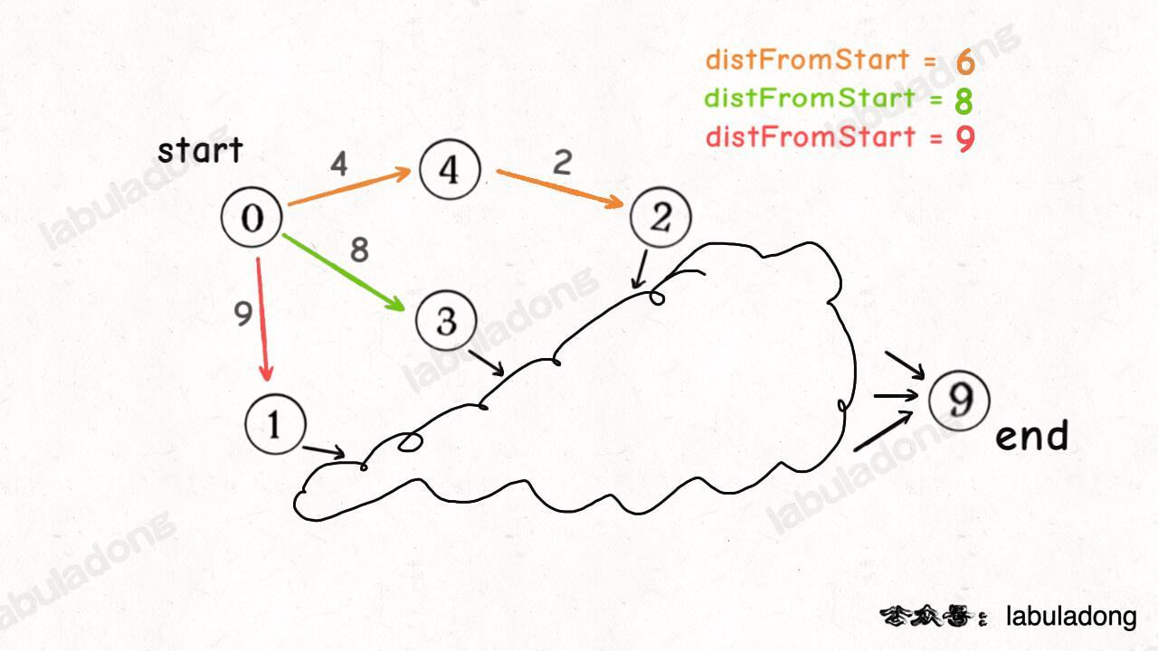
假设你当前只遍历了图中的这几个节点，那么你下一步准备遍历那个节点？这三条路径都可能成为最短路径的一部分，但你觉得哪条路径更有「潜力」成为最短路径中的一部分？

从目前的情况来看，显然橙色路径的可能性更大嘛，所以我们希望节点 2 排在队列靠前的位置，优先被拿出来向后遍历。

所以我们使用 PriorityQueue 作为队列，让 distFromStart 的值较小的节点排在前面，这就类似我们之前讲 贪心算法 说到的贪心思路，可以很大程度上优化算法的效率。

大家应该听过 Bellman-Ford 算法，这个算法是一种更通用的最短路径算法，因为它可以处理带有负权重边的图，Bellman-Ford 算法逻辑和 Dijkstra 算法非常类似，用到的就是普通队列，本文就提一句，后面有空再具体写。

接下来说第三个问题，如果只关心起点 start 到某一个终点 end 的最短路径，是否可以修改代码提升算法效率。

肯定可以的，因为我们标准 Dijkstra 算法会算出 start 到所有其他节点的最短路径，你只想计算到 end 的最短路径，相当于减少计算量，当然可以提升效率。

需要在代码中做的修改也非常少，只要改改函数签名，再加个 if 判断就行了：

// 输入起点 start 和终点 end，计算起点到终点的最短距离
int dijkstra(int start, int end, List<Integer>[] graph) {

    // ...

    while (!pq.isEmpty()) {
        State curState = pq.poll();
        int curNodeID = curState.id;
        int curDistFromStart = curState.distFromStart;

        // 在这里加一个判断就行了，其他代码不用改
        if (curNodeID == end) {
            return curDistFromStart;
        }

        if (curDistFromStart > distTo[curNodeID]) {
            continue;
        }

        // ...
    }

    // 如果运行到这里，说明从 start 无法走到 end
    return Integer.MAX_VALUE;
}

因为优先级队列自动排序的性质，每次从队列里面拿出来的都是 distFromStart 值最小的，所以当你第一次从队列中拿出终点 end 时，此时的 distFromStart 对应的值就是从 start 到 end 的最短距离。

这个算法较之前的实现提前 return 了，所以效率有一定的提高。

时间复杂度分析

Dijkstra 算法的时间复杂度是多少？你去网上查，可能会告诉你是 O(ElogV)，其中 E 代表图中边的条数，V 代表图中节点的个数。

因为理想情况下优先级队列中最多装 V 个节点，对优先级队列的操作次数和 E 成正比，所以整体的时间复杂度就是 O(ElogV)。

不过这是理想情况，Dijkstra 算法的代码实现有很多版本，不同编程语言或者不同数据结构 API 都会导致算法的时间复杂度发生一些改变。

比如本文实现的 Dijkstra 算法，使用了 Java 的 PriorityQueue 这个数据结构，这个容器类底层使用二叉堆实现，但没有提供通过索引操作队列中元素的 API，所以队列中会有重复的节点，最多可能有 E 个节点存在队列中。

所以本文实现的 Dijkstra 算法复杂度并不是理想情况下的 O(ElogV)，而是 O(ElogE)，可能会略大一些，因为图中边的条数一般是大于节点的个数的。

不过就对数函数来说，就算真数大一些，对数函数的结果也大不了多少，所以这个算法实现的实际运行效率也是很高的，以上只是理论层面的时间复杂度分析，供大家参考。

相关题目： LeetCode 743, 1631, 1514